
Quantum Measurement Methodology
Optically detected magnetic resonance (ODMR) encompasses a range of methodologies used to probe the spin properties of nitrogen-vacancy (NV) centers in diamond. Key measurement protocols include continuous-wave (CW) ODMR, spin relaxation (T₁), and spin coherence (T₂) experiments. These techniques not only assess the quality of NV centers but also form the foundation for quantum sensing applications. Learn more about these methodologies below: CW ODMR, T1 Relaxation, Rabi Oscillations, Hahn Echo, T2 Relaxation.
ODMR Setup
Adamas offers an ODMR measurement system: Here
An ODMR setup consists of a several components: optics for fluorescence imaging, light source, photodetector, microwave source, and computer for control and readout. Based on the way light and microwaves are administered, all the various optical spin experiments may be performed.
Adamas ODMR units are centered around a microscope to offer stability and flexibility for sample types with a movable stage. An LED light source provides optimal excitation of NV centers, however the optics can be readily configured for other ODMR systems. The light source is controllable via computer for CW or TTL triggered light pulsing. For microwave stimulation in ODMR measurements, a signal generator is used with high-frequency output up to 4 GHz. It provides substantial microwave output up to 16 dBm (44.7 mW) which may be further amplified. The delivery of microwave energy to the sample is achieved using a custom-designed omega-shaped loop antenna fabricated on a PCB board. With loop antennas, the samples are placed at the peak of the microwave field (B₁ field) and are easily accessible for optical illumination and detection on the microscope stage. A black box covering around the sample shields the measurement from ambient light and internal reflections. The microscope routes all optical signals for measurement via dedicated detector to convert light intensity into electrical signals. Data is acquired with a time resolution of 1 ns, ensuring high-resolution signal acquisition and precise temporal detail. This fast sampling capability enables effective noise reduction through averaging, contributing significantly to the accuracy and reliability of data acquisition in our experimental setup. Custom software provides ready operation of the entire instrument configuration.

CW Optically Detected Magnetic Resonance
Optically detected magnetic resonance (ODMR) of nanodiamonds with nitrogen-vacancy (NV) centers represents a cutting-edge technique in quantum sensing and materials characterization. NV centers, which are point defects within the diamond lattice, exhibit unique optical and magnetic properties that make them highly sensitive to their local environment. When exposed to microwave radiation, these NV centers experience changes in their fluorescence emission, which can be precisely measured to provide insights into various physical parameters.
The versatility of ODMR extends to probing the quality of the diamond crystal lattice, detecting lattice strain, and assessing environmental factors such as magnetic noise, temperature fluctuations, and external magnetic fields. This capability arises from the NV centers' robust fluorescence response and their dependence on quantum spin states. By applying continuous wave ODMR (CW-ODMR) techniques, researchers can obtain high-resolution spectra that reveal detailed information about the NV centers' spin dynamics and interactions with their surroundings. This makes ODMR nanodiamonds an invaluable tool for advanced quantum sensing applications and materials science.
A typical ODMR spectrum shown in Fig. 1 is centered around the NV zero field splitting parameter D at about 2.87 GHz. Recording the fluorescence intensity as a function of microwave frequency results in a drop in signal at this resonance frequency as compared to off-resonance frequencies. Due to strain and local charge splitting, two peak minima are observed with each being shifted from D symmetrically by a value E. Therefore, the distance between minima corresponds to 2 × E. The spectrum can be simulated by a superposition of two Lorentzian lines characterized by amplitude A, two centers D±E, and linewidth W representing the peak half-width at half-peak maximum (HWHM), using the formula: baseline – A × Σ 1 / [ 1+ ((frequency – (D±E))/W)²]. ODMR contrast can be extracted from the spectrum by normalization so that baseline corresponds to 100%. Then, contrast coincides with reduction of fluorescence to the minimum of normalized spectrum. More generally contrast = (baseline-minimum)/baseline 100 in %.
ODMR can be exploited for temperature, magnetic field and paramagnetic species measurements. See our recent papers on measurement of gaseous oxygen (doi.org/10.1002/adfm.76946).

Fig. 1.1. A typical NV ODMR spectrum with labeled parameters.
T1 Relaxation
T1 relaxation times represent the time scale over which the NV center(s) spin state returns to thermal equilibrium with its surroundings. This is also known as spin-lattice relaxation. This process is influenced by the local magnetic noise in the environment, which can be caused by unpaired electronic spins, paramagnetic impurities, or other defects in the diamond lattice. Such imperfections are often introduced during the manufacturing of diamond and the creation of NV centers. These interactions between the NV center and its noisy surroundings lead to energy dissipation, making T1 a valuable measure of the magnetic environment at the nanoscale. Fig. 4a and Fig. 4b shows the T1 protocol and a typical T1 decay trace, correspondingly. The T1 relaxation data acquisition protocol involves a series of light pulses structured as follows: an initialization pulse of length ∆tP is applied to establish a polarized state. This pulse is characterized by a rapid fluorescence signal jump, followed by a slower exponential build-up, typically occurring on a millisecond timescale. After a sufficiently long initialization period, typically 10 ms, a dark interval is introduced to allow for relaxation. Following the dark interval, a short detection pulse is applied with a controlled variable delay, typically ∆tD ranging from 100 μs to 200 μs. The signal is recorded during this period. The detection pulse signal undergoes processing through extrapolation fitting to a linear or exponential curve, enabling extraction of a signal value at the beginning of the pulse. This value represents a point in the T1 relaxation time at the specific detection pulse delay time. After a brief dark reset time, the sequence is repeated either for averaging purposes with the same delay time or to acquire the next relaxation point at successively increasing delay increments. There is a choice between keeping the reset time constant or the repetition period (T) constant between relaxation points.
Keeping the reset time constant enables faster data collection by dynamically adjusting the repetition time short enough to accommodate the current delay sequence. Conversely, maintaining a constant repetition time requires accommodating all pulse sequences and is limited by the longest delay time. While keeping the repetition time constant necessitates long reset times even for short delays, it is the best approach to ensure that the initialization states reach the same level of polarization for each sequence. This method is often the best way to prevent unwanted baseline drifts in the relaxation curve.
A typical relaxation curve follows approximately an exponential decay dependence of fluorescence signal on delay time between initialization and detection pulses. The curve can be modeled using a stretched exponential function of the form A × exp[-(delay/T1)ᵖ] + offset. Here, offset is the fluorescence signal level in the relaxed state, i.e., delay → ∞, A is the maximum increase of fluorescence level due to light polarization at the end of the initialization pulse, i.e., at the delay time zero, T1 is the relaxation constant, and ρ is the stretching exponent. Parameters are obtained by fitting a series of discrete points. It is advantageous to collect these data points with a parametric sampling scheme, where distance is kept constant along the relaxation curve instead of equidistant sampling on the delay axes. Such sampling provides a more accurate representation of the decay process and saves data acquisition time. If data are normalized so that the signal maximum at delay zero equals 100%, then parameter A equals the T1 contrast. More generally T1 contrast = A / (A + offset) x 100 in %.

Fig. 2.1. Schematic of T1 relaxation pulse protocol (a) and a typical T1 relaxation decay trace demarked with characteristic parameters (b)
Rabi Oscillations
Rabi oscillations represent the simplest experiment involving microwave pulses. The detection scheme is similar to that used in T1 relaxation measurements, but with one key difference: a progressively longer microwave pulse is inserted between the initialization and detection pulses.
The initial step in this experiment is determining the position of the resonance peak in the CW-ODMR spectrum. Once the peak’s frequency center is identified, the Rabi experiment can be initiated. To account for potential discrepancies—such as spectral broadening or shifts due to temperature or other factors—an optional optimization step can be performed to fine-tune the frequency center.
The primary challenge in the Rabi oscillations experiment lies in the disparity between the timescales of optical and microwave pulses. Optical detection pulses typically last a few milliseconds, and the overall time axis can extend to tens of milliseconds. In contrast, microwave pulses must be defined with durations on the order of tens of nanoseconds—a difference of up to six orders of magnitude. To address this, a two-channel Siglent AWG was used, allowing for precise synchronization between the optical and microwave pulse sequences with timing accuracy on the order of a few nanoseconds.
Once data is collected, the resulting Rabi oscillation curves can be modeled using damped harmonic functions, offering valuable insights into the spin dynamics of the system. The oscillation period allows estimation of the microwave B₁ field strength, while the damping rate provides an estimate of the effective transverse relaxation time, T₂*. Additionally, the number of harmonics required to accurately fit the data can be used to assess the polydispersity of the particles under study.
Figure 3.1 presents Rabi oscillations measured on a 150 µm NDNV sample subjected to a static bias magnetic field. The applied field shifts the resonance positions in the CW-ODMR spectrum, depending on its projection along specific NV axes (Figure 3.1, left). By selecting the resonance associated with a particular NV orientation, a distinct Rabi oscillation signal can be observed. It is important to note that Rabi oscillations represent the most basic spin coherence experiment. By linking the B₁ field strength to the microwave pulse duration, this measurement provides a critical baseline for more advanced pulsed experiments such as Ramsey interferometry and Hahn echo protocols.

Figure 3.1. Rabi oscillations experiment performed on 150 µm MDNV single crystal particle randomly oriented in the external magnetic field bias. CW spectrum with a typical 4 pairs resonance pattern associated with projections of external magnetic field onto four general NV axis orientations in a single crystal. By choosing a specific resonance peak, here the 5th line from left, we can isolate single NV axis and analyze Rabi oscillations associated with it.
Hahn Echo
Similarly to the Rabi oscillations protocol, the Hahn echo experiment extends the microwave pulse sequence inserted between the optical initialization and detection pulses. However, instead of a single microwave pulse, a three-pulse sequence π⁄2 – π – π⁄2 is used, where the π pulse length is calibrated from the period of the Rabi oscillations (2 π representing the oscillation period in time units). After building up spin polarization during the initialization phase, a first π⁄2 pulse rotates the polarization vector on the Bloch sphere from the z axis to the xy-plane. Following a fixed evolution time t₁, a π pulse is applied, which flips the dephasing spins along the x axis, effectively reversing their order. As a result, spins that were dephasing faster now lag behind by time t₁. Finally, a third π⁄2 pulse is applied at time t₂ after the previous pulse, projecting the recovered spin coherence back onto the measurable z axis (Figure 4.1). Due to symmetry, the fluorescence signal (reflecting spin polarization) is expected to reach a maximum when t₂ = t₁. Hence sweeping t₂ around t₁ results in a detectable Gaussian-shaped echo (Figure 5.1 top trace window). In this way, the influence of static or low frequency inhomogeneities (but not rapid stochastic perturbations) that cause spin dephasing is eliminated from the echo amplitude. The overall rate of transversal dephasing T₂* is still visible in the echo and can be estimated from the echo width.
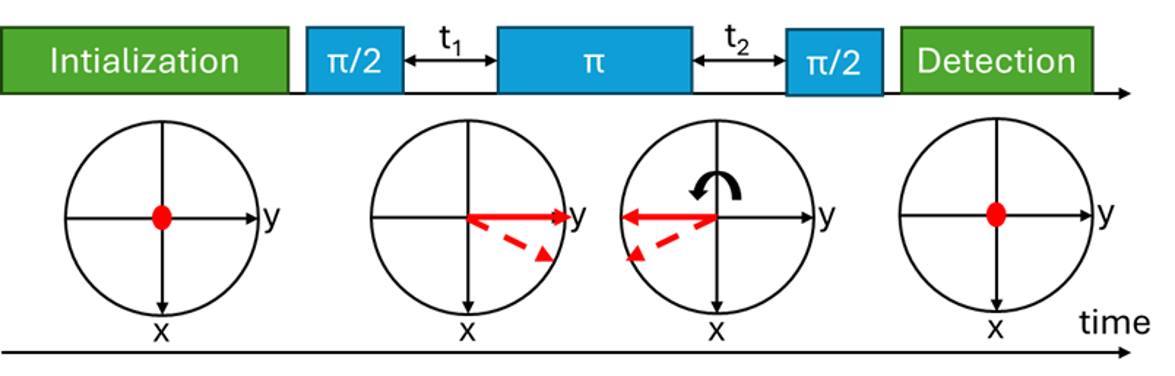
Figure 4.1. Schematic representation of the Hahn Echo protocol. In green depicted initialization and detection light pulses, in blue the microwave pulses followed by the polarization vector representation on the Bloch sphere in red.
T2 Relaxation
Since static, primarily instrumental inhomogeneities are canceled out in the amplitude of the Hahn echo, the sequence allows us to probe the stochastic (time-varying) component of transverse relaxation, quantified by T₂. In such an experiment, the evolution times t₁ and t₂ are kept equal, and the total time t₁ = t₂ is gradually increased. The echo amplitude is measured at the total evolution time t=2t₁. This relaxation curve reveals extended relaxation times compared to methods that do not refocus static dephasing. Such experiments are practical only in well-oriented samples. Even in single-crystal NV diamond, four distinct NV axis orientations are present. Each axis experiences a different projection of the microwave B₁ field, which leads to axis-specific variations in the effective microwave pulse durations. To overcome this, it is advantageous to apply an external static magnetic field bias to lift the degeneracy of the NV resonances. The Zeeman splitting caused by this bias separates the resonance frequencies of the different NV orientations according to the projection of the bias field onto each NV axis (analogous to the B₁ field projection). By tuning the microwave frequency to a single, isolated resonance peak, one can selectively address NV centers aligned along a specific axis, ensuring consistent and well-defined pulse durations. However, in diamonds, the situation is more complex because of the presence of nearby 13C nuclei. With a natural abundance of approximately 1.1%, each 13C nucleus possesses a nuclear spin of ½, which generates a local magnetic field at the position of a nearby NV⁻ center. Under an external magnetic field B₀, these nuclear spins precess at their Larmor frequency fL=γ₁₃C*B₀, where γ₁₃C=1.0705 kHz/G is the gyromagnetic ratio of the 13C nucleus. Because the total magnetic field experienced by an NV⁻ center is periodically modulated by these precessing nuclear spins, it is intuitive to expect a corresponding modulation in the echo amplitude at the same frequency. A more rigorous treatment shows that this behavior arises from mutual “hyperfine” interaction: not only do the nuclear spins influence the NV⁻ electronic spin, but the NV⁻ also perturbs the nuclear spin states. For more frequented distant 13C position, the hyperfine coupling becomes weak, and the modulation frequency approaches the bare Larmor frequency f. An important consideration is that the T₂ relaxation signal is typically plotted as a function of the total evolution time t = 2*t₁. Because the Hahn echo experiment effectively mirrors the phase accumulation between the two t₁ intervals, the full acquired phase (and thus the observed modulation period) is doubled. As a result, the observed modulation frequency in the T₂ relaxation curve is half the nuclear Larmor frequency fL. This fact is crucial when estimating the magnetic field strength from the modulation periodicity.
In an ensemble measurement only a fraction of NV⁻ centers undergo state flips due to interaction with nearby 13C nuclei. Therefore, the total echo signal consists of both modulated and unmodulated components. The modulation amplitude typically decays at a different rate, often faster than the bulk T₂ envelope. This composite behavior can be modeled as a superposition of an exponentially decaying harmonic term and the main T₂ envelope:

where: A is the unmodulated relaxation amplitude fraction, Am is the amplitude of the modulated component, τm is its modulation decay constant, fm≈fL/2 is the apparent modulation frequency, andT2 is the overall relaxation time with stretching exponent p (typically 1≤p≤2).
Figure 5.1. shows a simultaneous analysis of the Hahn echo and T₂ relaxation performed on an optical-grade [100]-cut diamond plate. Under an external static magnetic bias field oriented along a [111] NV axis, the sample exhibits a greatly extended T₂ relaxation time of approximately 446 µs (light blue windows). This is especially notable when contrasted with the much shorter dephasing T₂* time, measured from the echo width at approximately 0.08 µs (purple windows).

Fig. 5.1. The Hahn echo and T2 relaxation curves.